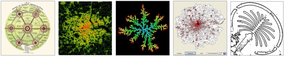
 A rank clock is a device for visualising the changes over time in the rank order in any set of objects where the ordering is usually from large to small. The size of cities, of firms, the distribution of incomes, heights of skyscrapers and sizes of nodes in social networks display highly ordered distributions. If you rank these phenomena from largest to smallest, the objects follow a power law over much of their range, or at least a log normal distribution, with a power law in their upper tail.
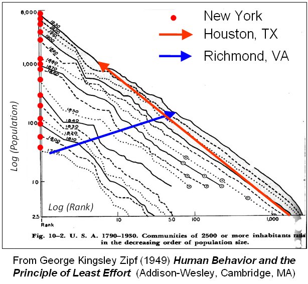
In fact for cities and other phenomena such as the distribution of word frequencies, George Kingsley Zipf as long ago as the 1930s characterised such distributions as characterising pure power laws in which the size of an object seemed to approximate the largest object in the set divided by the rank of the object in question. Such strict power laws in fact seem to be the exception rather than the rule but many such rank size distributions seem to follow such laws in their upper tail, and hence these are taken as signs of system stability, self-organisation and universality.
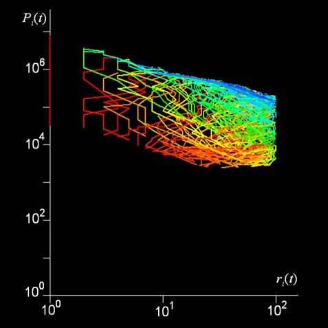
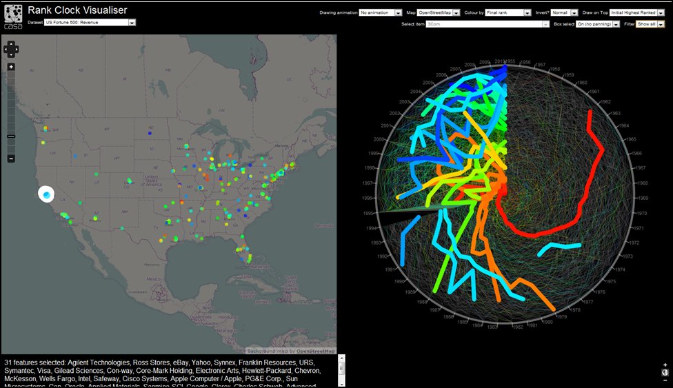
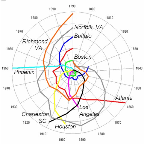 Zipf Plot Rank Clock Rank Space Clock Trajectories
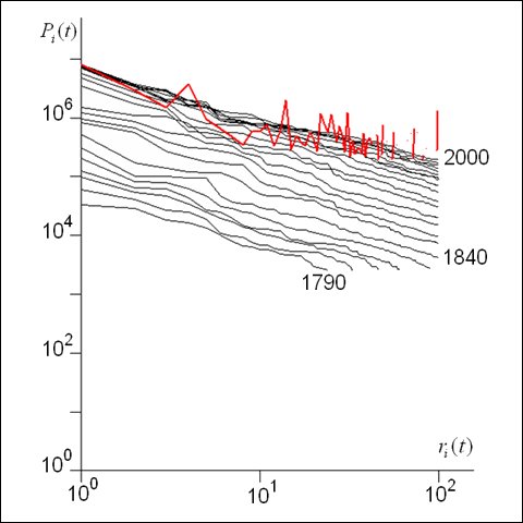
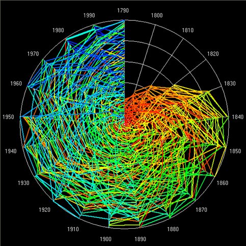
However despite the fact that such distributions are so regular even through time, when one examines how objects within these distributions change over time, it is quite clear that somehow these systems remain stable at the aggregate level but with objects which composes them shifting quite dramatically from time period to time period. The Rank Clock is a device that shows how such distributions change over time and it is a natural complement to the rank size distribution which is called a Zipf Plot. The rank clock relates time to rank, while the Zipf plot relates size to rank. Ways of visualising how size in a rank clock and time in a Zipf plot can be added relate to various animations which we are working on, Ollie O’Brien and Martin Austwick are working with me on such visualisations and in time, we will put up a web site to make this media accessible. Here is a glimpse.
We developed a program for plotting these clocks back in 2006 when I first published the Nature paper on this, and there is some supplementary information too, that is on the Nature web site but if you want it directly, click here. The software can be downloaded in stripped down form with data for the top 100 cities in the US urban system for the decades from 1790 to 2000.
 Download software as a zip file. Don’t forget that this software is for Windows and won’t run on a Mac. If on a Mac, you will have to be content with viewing our demos, reading the paper and getting onto Ollie O’Brien’s test web site, where you can play around with some examples, but again if on the web site, use Google Chrome as this is best for the vector graphics.
We have also examined the UK urban system from 1901 to 2001, the World System from 430BCE to 2000, and the Ancient World System from 3700BCE to 1000BCE. All these examples show quite regular stability in rank size at the aggregate Zipf Plot level but much greater volatility in terms of the Rank Clocks and this in an of itself throws grave doubt on the issue of universality and regularity in such systems. Moreover it opens up once again the paradox of why systems show such regularity at the macro level when everything is changing at the micro level. Other examples we have looked at are skyscrapers, firm expenditures and profits for the top 100 firms in the US (from the Fortune 500), species size in ecological communities, and the size and duration of wars in the last 50 years. Anything that scales where the scaling changes over time is fair game for this kind of visualisation.
We conclude with a demo of the clock for the example of skyscrapers in New York City but we are going to put a lot of different demos here ultimately once we get our act together as this is an active project.
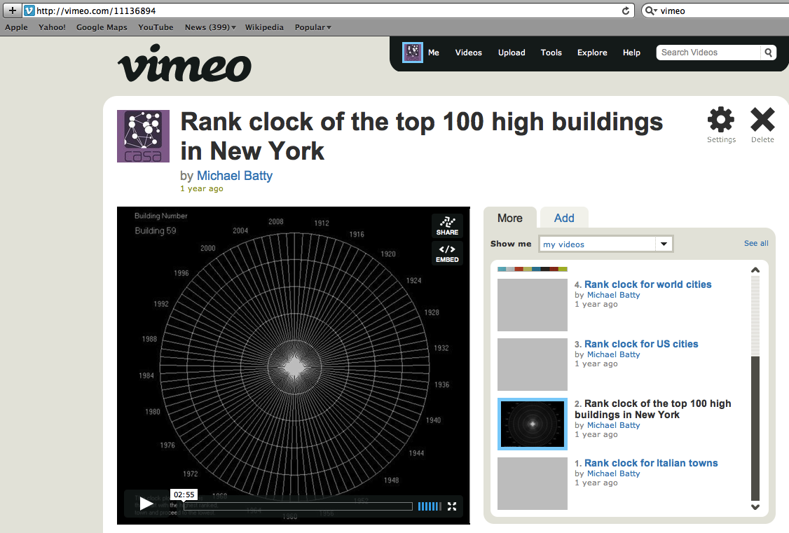 Click left to load the movie. All you need to know now is that what you are seeing is first all the trajectories being plotted, then one by one for each building starting with the one that is highest in 1909 and then the next highest and so on until the next time point is reached at 1910 and so on …. The trajectories build up and spiral out as very few buildings get bigger with time.
Look at the publications (articles) section of this web site to find some more papers on this kind of visualisation.