
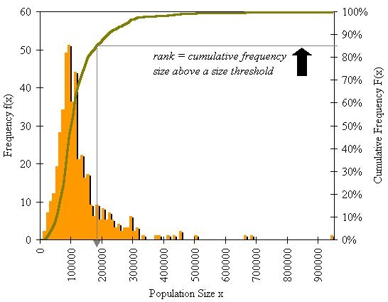
 If we look at the population sizes x of the objects which define cities – such as their entire populations or any other measure that define their size – very often these sizes follow a frequency distribution f(x) which declines with size; that is as cities get larger they are less frequent – there are less of them. If we then examine the cumulative distribution of cities F(x) these will follow not the S shaped curve that define a normal distribution but a curve whose
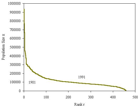 rate of change declines as the size of cities gets greater. We can then extract from this the counter cumulative distribution 1-F(x) which in fact is also a skew distribution where we plot city size against their rank r(x) (which is the counter cumulative frequency) which shows that the rank of a city declines inversely with its size.
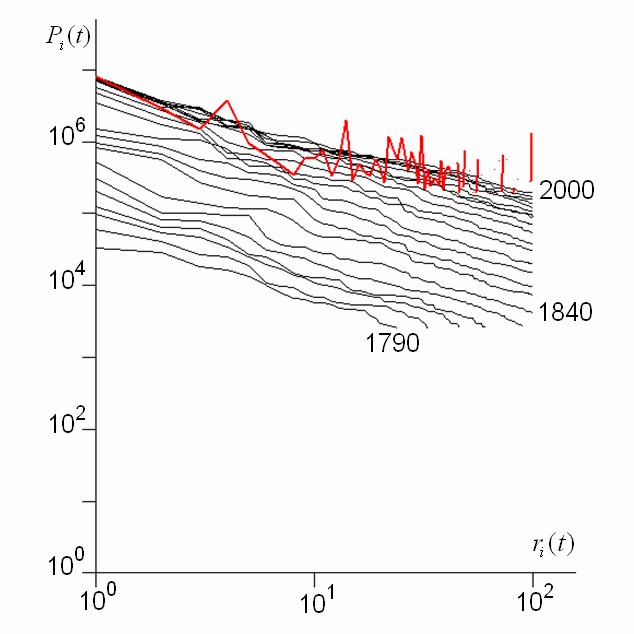
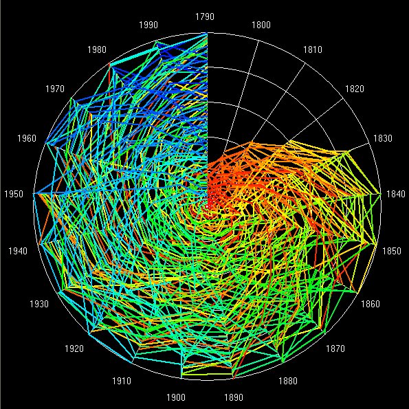
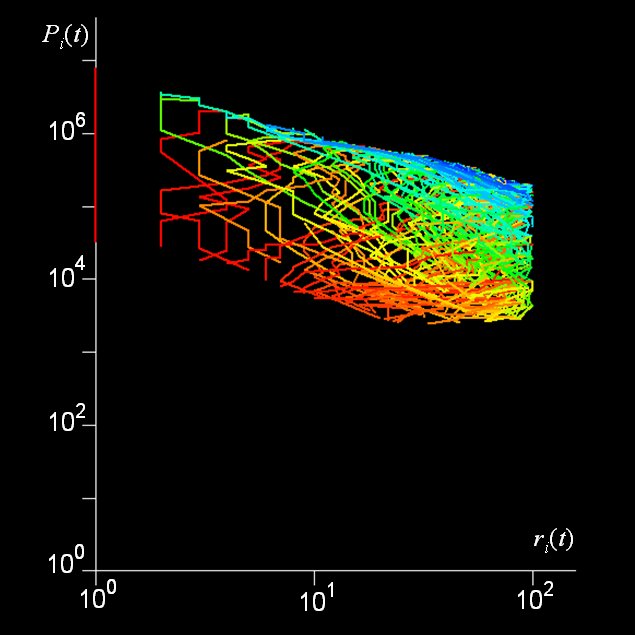
Now these kinds of distributions are often lognormal but a lognormal can usually be approximated for its largest values of size by a power law. Power laws are scaling, thus city size distributions might be said to be fractal. So the argument goes and it is an intriguing but perplexing one. We have examined many city size distributions for different systems and also looked at these over time. They tend to be scaling and are also extremely regular from time period to time period. But if we look at the ranks of the individual objects making up such distributions, these ranks change rather frequently. Thus aggregate stability flies in the face of micro-volatility as the following plot, clock and rank space show for changes in rank and size of the top 100 cities in the US from 1790 to 2000.
An early paper, maybe our first in 2003, which is in our Advanced Spatial Analysis book, written with Naru Shiode and entitled “Population Growth Dynamics in Cities, Countries and Communication Systems” provides a gentle introduction to these ideas. You can download it by clicking here.
UNDER DEVELOPMENT …..